推荐学习书目
› Learn Python the Hard Way
Python Sites
› PyPI - Python Package Index
› http://diveintopython.org/toc/index.html
› Pocoo
值得关注的项目
› PyPy
› Celery
› Jinja2
› Read the Docs
› gevent
› pyenv
› virtualenv
› Stackless Python
› Beautiful Soup
› 结巴中文分词
› Green Unicorn
› Sentry
› Shovel
› Pyflakes
› pytest
Python 编程
› pep8 Checker
Styles
› PEP 8
› Google Python Style Guide
› Code Style from The Hitchhiker's Guide

这是一个创建于 2610 天前的主题,其中的信息可能已经有所发展或是发生改变。
python 之数据分析利器
这一部分主要学习 pandas 中基于前面两种数据结构的基本操作。
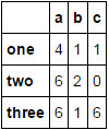
设有 DataFrame 结果的数据 a 如下所示:
一、查看数据(查看对象的方法对于 Series 来说同样适用)
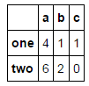
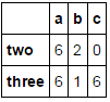
1.查看 DataFrame 前 xx 行或后 xx 行 a=DataFrame(data); a.head(6)表示显示前 6 行数据,若 head()中不带参数则会显示全部数据。 a.tail(6)表示显示后 6 行数据,若 tail()中不带参数则也会显示全部数据。
import pandas as pd
import numpy as np
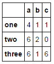
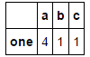
a=pd.DataFrame([[4,1,1],[6,2,0],[6,1,6]],index=['one','two','three'],columns=['a','b','c'])
a
a.head(2)
a.tail(2)
2.查看 DataFrame 的 index , columns 以及 values a.index ; a.columns ; a.values 即可
a.index
Index([u'one', u'two', u'three'], dtype='object')
a.columns
Index([u'a', u'b', u'c'], dtype='object')
a.values
array([[4, 1, 1],
       [6, 2, 0],
       [6, 1, 6]])
3.describe()函数对于数据的快速统计汇总
a.describe()对每一列数据进行统计,包括计数,均值, std ,各个分位数等。
a.describe
<bound method DataFrame.describe of        a  b  c
one    4  1  1
two    6  2  0
three  6  1  6>
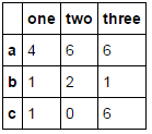
4.对数据的转置
a.T
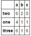
5.对轴进行排序 a.sort_index(axis=1,ascending=False);其中 axis=1 表示对所有的 columns 进行排序,下面的数也跟着发生移动。后面的 ascending=False 表示按降序排列,参数缺失时默认升序。
a.sort_index(axis=1,ascending=False);
a
6.对 DataFrame 中的值排序 a.sort(columns=’ x ’) 即对 a 中的 x 这一列,从小到大进行排序。注意仅仅是 x 这一列,而上面的按轴进行排序时会对所有的 columns 进行操作。
a.sort(columns='c')
二、选择对象
1.选择特定列和行的数据 a[‘ x ’] 那么将会返回 columns 为 x 的列,注意这种方式一次只能返回一个列。 a.x 与 a[‘ x ’]意思一样。
取行数据,通过切片[]来选择 如: a[0:3] 则会返回前三行的数据。
a['a']
one      4
two      6
three    6
Name: a, dtype: int64
a[0:2]

2.通过标签来选择 a.loc[‘ one ’]则会默认表示选取行为’ one ’的行;
a.loc[:,[‘ a ’,’ b ’] ] 表示选取所有的行以及 columns 为 a,b 的列;
a.loc[[‘ one ’,’ two ’],[‘ a ’,’ b ’]] 表示选取’ one ’和’ two ’这两行以及 columns 为 a,b 的列;
a.loc[‘ one ’,’ a ’]与 a.loc[[‘ one ’],[‘ a ’]]作用是一样的,不过前者只显示对应的值,而后者会显示对应的行和列标签。
3.通过位置来选择
这与通过标签选择类似 a.iloc[1:2,1:2] 则会显示第一行第一列的数据;(切片后面的值取不到)
a.iloc[1:2] 即后面表示列的值没有时,默认选取行位置为 1 的数据;
a.iloc[[0,2],[1,2]] 即可以自由选取行位置,和列位置对应的数据。
a.iloc[1:2,1:2]

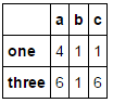
4.使用条件来选择 使用单独的列来选择数据 a[a.c>0] 表示选择 c 列中大于 0 的数据
a[a.c>0]
使用 where 来选择数据 a[a>0] 表直接选择 a 中所有大于 0 的数据
a[a>0]
使用 isin()选出特定列中包含特定值的行 a1=a.copy() a1[a1[‘ one ’].isin([‘ 2 ′,’ 3 ′])] 表显示满足条件:列 one 中的值包含’ 2 ’,’ 3 ’的所有行。
a1=a.copy()
a1[a1['a'].isin([4])]
三、设置值(赋值)
赋值操作在上述选择操作的基础上直接赋值即可。 例 a.loc[:,[‘ a ’,’ c ’]]=9 即将 a 和 c 列的所有行中的值设置为 9 a.iloc[:,[1,3]]=9 也表示将 a 和 c 列的所有行中的值设置为 9
同时也依然可以用条件来直接赋值
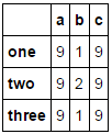
a[a>0]=-a 表示将 a 中所有大于 0 的数转化为负值
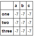
a.loc[:,['a','c']]=9
a
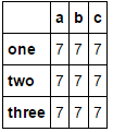
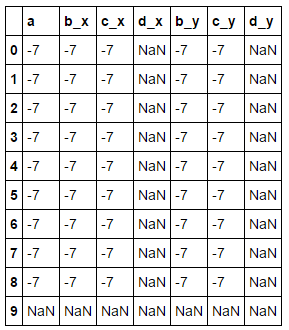
a.iloc[:,[0,1,2]]=7
a
a[a>0]=-a
a
四、缺失值处理
在 pandas 中,使用 np.nan 来代替缺失值,这些值将默认不会包含在计算中。
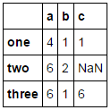
1.reindex()方法 用来对指定轴上的索引进行改变 /增加 /删除操作,这将返回原始数据的一个拷贝。 a.reindex(index=list(a.index)+[‘ five ’],columns=list(b.columns)+[‘ d ’])
a.reindex(index=[‘ one ’,’ five ’],columns=list(b.columns)+[‘ d ’])
即用 index=[]表示对 index 进行操作, columns 表对列进行操作。
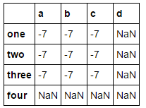
b=a.reindex(index=list(a.index)+['four'],columns=list(a.columns)+['d'])
c=b.copy()
c
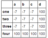
2.对缺失值进行填充 a.fillna(value=x) 表示用值为 x 的数来对缺失值进行填充
b.fillna(value=100)
3.去掉包含缺失值的行 a.dropna(how=’ any ’) 表示去掉所有包含缺失值的行
c.dropna(how='any')

五、合并
1.contact contact(a1,axis=0/1 , keys=[‘ xx ’,’ xx ’,’ xx ’,…]),其中 a1 表示要进行连接的列表数据,axis=1 时表横着对数据进行连接。 axis=0 或不指定时,表将数据竖着进行连接。 a1 中要连接的数据有几个则对应几个 keys ,设置 keys 是为了在数据连接以后区分每一个原始 a1 中的数据。
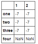
例: a1=[b[‘ a ’],b[‘ c ’]] result=pd.concat(a1,axis=1 , keys=[‘ 1 ′,’ 2 ’])
a1=[b['a'],b['c']]
d=pd.concat(a1,axis=1,keys=['1','2'])
d
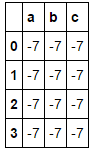
2.Append 将一行或多行数据连接到一个 DataFrame 上 a.append(a[2:],ignore_index=True) 表示将 a 中的第三行以后的数据全部添加到 a 中,若不指定 ignore_index 参数,则会把添加的数据的 index 保留下来,若 ignore_index=Ture 则会对所有的行重新自动建立索引。
a.append(a[2:],ignore_index=True)
3.merge 类似于 SQL 中的 join 设 a1,a2 为两个 dataframe,二者中存在相同的键值,两个对象连接的方式有下面几种: (1)内连接, pd.merge(a1, a2, on=’ key ’) (2)左连接, pd.merge(a1, a2, on=’ key ’, how=’ left ’) (3)右连接, pd.merge(a1, a2, on=’ key ’, how=’ right ’) (4)外连接, pd.merge(a1, a2, on=’ key ’, how=’ outer ’) 至于四者的具体差别,具体学习参考 sql 中相应的语法。
pd.merge(b,c,on='a')
六、分组( groupby )
用 pd.date_range 函数生成连续指定天数的的日期 pd.date_range(‘ 20000101 ’,periods=10)
def shuju():
data={
‘ date ’:pd.date_range(‘ 20000101 ’,periods=10),
‘ gender ’:np.random.randint(0,2,size=10),
‘ height ’:np.random.randint(40,50,size=10),
‘ weight ’:np.random.randint(150,180,size=10)
}
a=DataFrame(data)
print(a)
date gender height weight
0 2000-01-01 0 47 165
1 2000-01-02 0 46 179
2 2000-01-03 1 48 172
3 2000-01-04 0 45 173
4 2000-01-05 1 47 151
5 2000-01-06 0 45 172
6 2000-01-07 0 48 167
7 2000-01-08 0 45 157
8 2000-01-09 1 42 157
9 2000-01-10 1 42 164
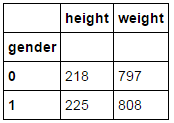
用 a.groupby(‘ gender ’).sum()得到的结果为: #注意在 python 中 groupby(” xx)后要加 sum(),不然显示
不了数据对象。
gender height weight
0 256 989
1 170 643
此外用 a.groupby(‘ gender ’).size()可以对各个 gender 下的数目进行计数。
所以可以看到 groupby 的作用相当于: 按 gender 对 gender 进行分类,对应为数字的列会自动求和,而为字符串类型的列则不显示;当然也可以同时 groupby([‘ x1 ′,’ x2 ’,…])多个字段,其作用与上面类似。
a2=pd.DataFrame({
        'date':pd.date_range('20000101',periods=10),
        'gender':np.random.randint(0,2,size=10),
        'height':np.random.randint(40,50,size=10),
        'weight':np.random.randint(150,180,size=10)
    })
print(a2)

        date  gender  height  weight
0 2000-01-01       0      43     151
1 2000-01-02       1      40     171
2 2000-01-03       1      49     169
3 2000-01-04       1      48     165
4 2000-01-05       0      42     159
5 2000-01-06       1      48     152
6 2000-01-07       0      48     154
7 2000-01-08       1      40     151
8 2000-01-09       0      41     158
9 2000-01-10       0      44     175
a2.groupby('gender').sum()
七、 Categorical 按某一列重新编码分类
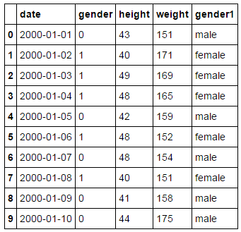
如六中要对 a 中的 gender 进行重新编码分类,将对应的 0 , 1 转化为 male , female ,过程如下:
a[‘ gender1 ’]=a[‘ gender ’].astype(‘ category ’)
a[‘ gender1 ’].cat.categories=[‘ male ’,’ female ’] #即将 0 , 1 先转化为 category 类型再进行编码。
print(a)得到的结果为:
date gender height weight gender1
0 2000-01-01 1 40 163 female
1 2000-01-02 0 44 177 male
2 2000-01-03 1 40 167 female
3 2000-01-04 0 41 161 male
4 2000-01-05 0 48 177 male
5 2000-01-06 1 46 179 female
6 2000-01-07 1 42 154 female
7 2000-01-08 1 43 170 female
8 2000-01-09 0 46 158 male
9 2000-01-10 1 44 168 female
所以可以看出重新编码后的编码会自动增加到 dataframe 最后作为一列。
a2['gender1']=a2['gender'].astype('category')
a2['gender1'].cat.categories=['male','female']
a2
八、相关操作
描述性统计: 1.a.mean() 默认对每一列的数据求平均值;若加上参数 a.mean(1)则对每一行求平均值;
a2.mean()
gender      0.5
height     44.3
weight    160.5
dtype: float64
2.统计某一列 x 中各个值出现的次数: a[‘ x ’].value_counts();
a2['height'].value_counts()
0    64.666667
1    70.666667
2    73.000000
3    71.333333
4    67.000000
5    67.000000
6    67.333333
7    64.000000
8    66.333333
9    73.000000
dtype: float64
3.对数据应用函数 a.apply(lambda x:x.max()-x.min()) 表示返回所有列中最大值-最小值的差。
d.apply(lambda x:x.max()-x.min())
1    0
2    0
dtype: float64
4.字符串相关操作 a[‘ gender1 ’].str.lower() 将 gender1 中所有的英文大写转化为小写,注意 dataframe 没有 str 属性,只有 series 有,所以要选取 a 中的 gender1 字段。
a2['gender1'].str.lower()
0      male
1    female
2    female
3    female
4      male
5    female
6      male
7    female
8      male
9      male
Name: gender1, dtype: object
九、时间序列
在六中用 pd.date_range(‘ xxxx ’,periods=xx,freq=’ D/M/Y ….’)函数生成连续指定天数的的日期列表。 例如 pd.date_range(‘ 20000101 ’,periods=10),其中 periods 表示持续频数; pd.date_range(‘ 20000201 ′,’ 20000210 ′,freq=’ D ’)也可以不指定频数,只指定其实日期。
此外如果不指定 freq ,则默认从起始日期开始,频率为 day 。其他频率表示如下:
print(pd.date_range('20000201','20000210',freq='D'))
DatetimeIndex(['2000-02-01', '2000-02-02', '2000-02-03', '2000-02-04',
               '2000-02-05', '2000-02-06', '2000-02-07', '2000-02-08',
               '2000-02-09', '2000-02-10'],
              dtype='datetime64[ns]', freq='D')
print(pd.date_range('20000201',periods=5))
DatetimeIndex(['2000-02-01', '2000-02-02', '2000-02-03', '2000-02-04',
               '2000-02-05'],
              dtype='datetime64[ns]', freq='D')
十、画图(plot)
在 pycharm 中首先要: import matplotlib.pyplot as plt
a=Series(np.random.randn(1000),index=pd.date_range(‘ 20100101 ’,periods=1000))
b=a.cumsum()
b.plot()
plt.show() #最后一定要加这个 plt.show(),不然不会显示出图来。
import matplotlib.pyplot as plt
a=pd.Series(np.random.randn(1000),index=pd.date_range('20150101',periods=1000))
b=a.cumsum()
b.plot()
plt.show()
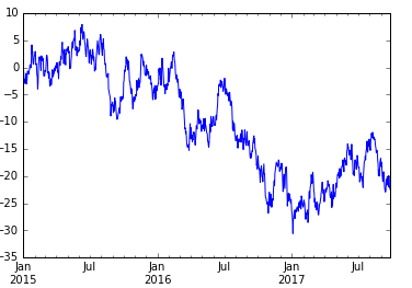
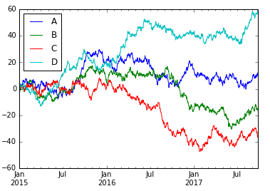
也可以使用下面的代码来生成多条时间序列图:
a=DataFrame(np.random.randn(1000 , 4),index=pd.date_range(‘ 20100101 ’,periods=1000),columns=list(‘ ABCD ’))
b=a.cumsum()
b.plot()
plt.show()
a=pd.DataFrame(np.random.randn(1000,4),index=pd.date_range('20150101',periods=1000),columns=list('ABCD'))
b=a.cumsum()
b.plot()
plt.show()
以上代码不想自己试一试吗?
镭矿raquant提供jupyter在线练习学习python的机会,无需安装python即可运行python程序。


